不好意思,还是没看明白,不过还是谢谢你了.
by the two adjacent peaks of the transmission parameter. The final geometry is shown in Figure 1.
Figure 1: Final geometry. Note, that the capacitive cross-coupling is made inactive by minimizing its length
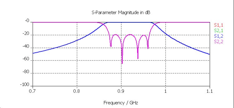
Figure 2: Typical Chebyshev- response after completion of the tuning process
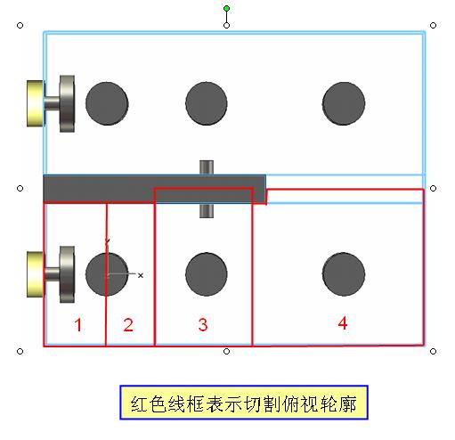
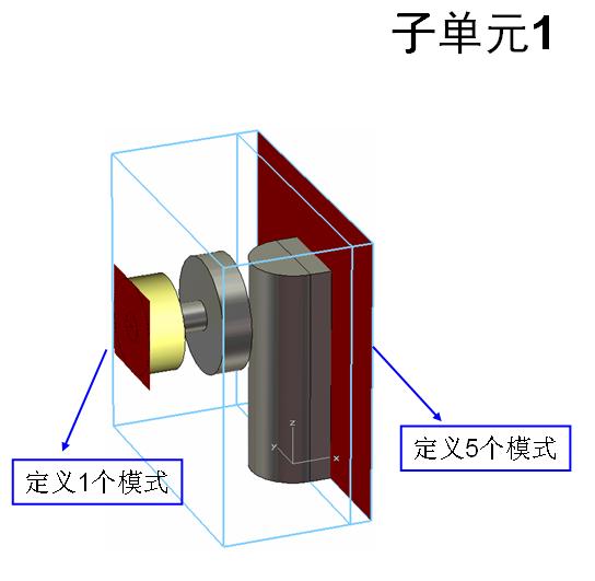
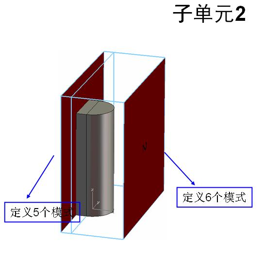
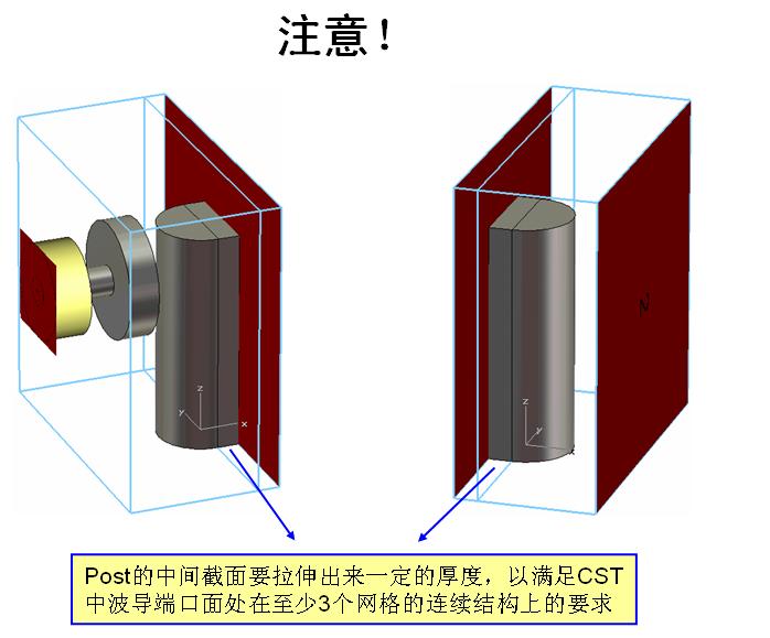
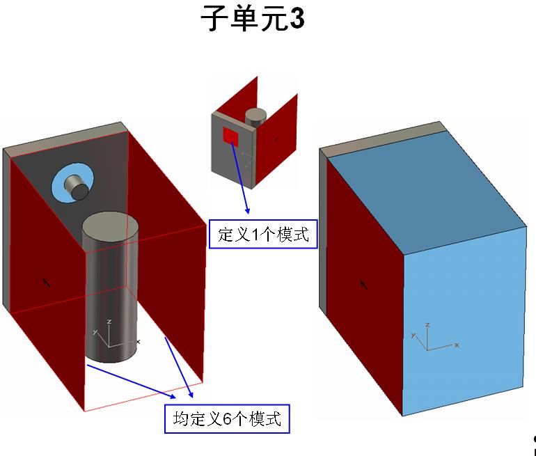
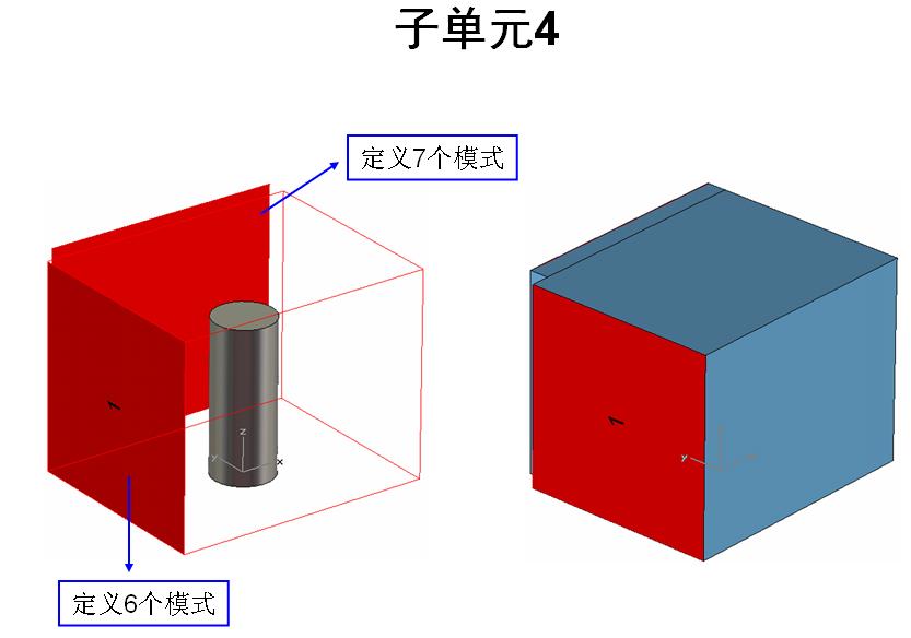
Instead of performing the optimization with the complete filter, the model was split up into several sub-sections. wWaveguide ports considering a sufficiently large number of modes are assigned at the intersections . CST MWS is used to compute the required S-parameters. Since the number of meshcells of the submodels is small compared to a complete model the runtimes are extremely short, thus the meshdensity can be increased to achieve higher accuracy. Since frequencies below cutoff are considered it is advisable to use the Frequency Domain solver within CST MWS: here the Model order Reduction solver (MOR) was used. Figure 3 illustrates this procedure: Only four submodels are required to describe the complete filter.
Figure 3: Definition of the sub-models: At the common interfaces between the sub-models waveguide ports are assigned (not shown here)
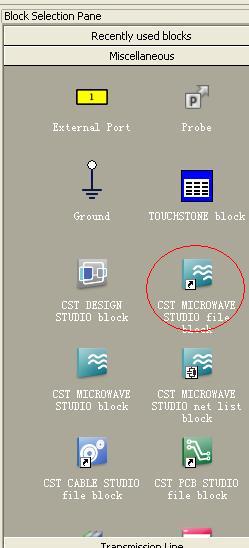
The sub-models are loaded into CST DS and linked together. The local sub-model parameters can be accessed and assigned to a global CST DS parameter. These parameters can be used in an optimization process. CST DS uses an interpolation scheme in order to avoid numerous recomputations of S-parameters for individual setups required by the optimizer.
Figure 4: CST MWS submodels and their connections via modes. Note the link to global CST DS parameters
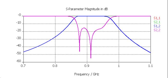
Figure 5: S-Parameter view of CST DS results
In a next step, the length of the capacitive cross-coupling stub is enlarged to increase the coupling bandwidth for a quadruplet type behaviour described in [3] and [4].
Figure 6: Enlarging the length of the stub reinforces the coupling bandwidth
Figure 7: The transmission zeros are still in the upper stopband indicating that the coupling is too small. Shown here is also a comparison between a complete model and a sub-model result using CST DS
Finally, the cross-coupling is further increased, resulting in a symmetric location of the transmission zeros above and below the passband. The next two figures show the geometry and the respective S-parameters.
Figure 8: Further enlargement of the cross coupling stub
Figure 9: Results of the CST DS model: Two transmission zeros appear above and below passband. Adding a diagonally positioned coupling would allow a more symmetric rejection shape
References:
[1] John B. Ness: "A Unified Approach to the Design, Measurement, and Tuning of Coupled-Resonator Filters", IEEE Trans. on MW Theor. and Tech., Vol 46, No 4, April 1998
[2] Peter Martin, John B. Ness: "Coupling Bandwidth and Reflected Group Delay Characterization of MW Bandpass Filters", Applied MW&Wireless, Vol 11, No 5.
[3] Raph Levy: "Filters with Single Transmission Zeros at Real or Imaginary Frequencies", IEEE Trans. on MW Theor. and Techn., Vol. MTT-24, No 4, April 1976
[4] Ralph Levy, Peter Petre: "Design of CT and CQ Filters Using Approximation and Optimization", IEEE Trans. on MW Theor. and Techn., Vol 49, No. 12, Dec. 2001
Appendix:
A bandpass filter can simply be described by low-pass prototype LC elements and by coupling coefficients of the inverter coupled filter. Approximation techniques can be used to get good initial values of the lumped elements [4] to find an optimal overall performance in a consecutive optimization loop. The cross-couplings requires slight changes of the theoretical Chebychev values resulting in very small geometrical modifications. A The next figure shows the equivalent network including also a cross-coupling admittance inverter with a negative C across the nodes 2 and 5.
Figure 10: Circuit elements for inverter coupled filter structures
Figure 11: Optimized filter response of the bandpass filter within CST DS
Figure 12: Parameter list of optimized LC lumped element values
CST Article "Six-Pole Bandpassfilter with Single Cross-Coupling"
last modified 26. Mar 2007 9:43
printed 9. Jan 2009 5:55, Article ID 136
URL:
http://imw.mwhrf.com/redirect.php?tid=17725&goto=lastpost
All rights reserved.
Without prior written permission of CST, no part of this publication may be reproduced by any method, be stored or transferred into an electronic data processing system, neither mechanical or by any other method.
Download as PDF
Article ID: 136 Last modified: 26. Mar 2007 9:43我用时延仿真了一个4腔的滤波器,第一个图为其结构,第二个为cst后处理时延调节的结果(results-template based。。-1dresult-group delay time),第三个图为整体优化的结果,用sub-models的结果实在是差,而且用DS来优化时机器运行缓慢,可能是我的设置有问题,所以请有建好sub-models模型的发上来学习下(我就是根据上面的pdf文档来仿真的)


[
本帖最后由 zhca 于 2009-1-12 08:48 编辑 ]
